

本記事はアフィリエイト広告(PR)を含みます
前回の記事では
- Stable Diffusion
- BiRefNet
- Ollama
を組み合わせることで画像生成~COCOフォーマットのデータセットを一括で作成する手順について解説しました。

今回は、実際にAI画像のみで作成したデータセットを読み込み、画像分類を試していきたいと思います。

1. 前提条件
今回検証を行うPCのスペックはこちらです。
Google Colaboなどのクラウド環境ではなくローカル環境で行います。
| 項目 | 環境 |
|---|---|
| OS | Windows 11 Home |
| CPU | Intel Core Ultra 7 265KF |
| GPU | NVIDIA GeForce RTX 5070 Ti |
| VRAM | 16GB |
| メモリ | DDR5 32GB(16GB × 2) |
| SSD | Samsung 990 PRO 2TB(PCIe 4.0 NVMe M.2) |

今回の学習では犬と猫の2種類を分類させるように学習させます。
また、分類用のモデルについては以下の4種類それぞれで学習し、比較してみます。
- VGG16
- ResNet50
- EfficientNet
- ConvNeXt
なお、ImageNetで学習されたモデルは既に犬と猫が学習されてしまっているので、今回はファインチューニングは行わず、1から学習させて精度を確認します。
2. データセットクラス
まずはCOCOフォーマットのデータセットを読み込むためのデータセットクラスを実装します。
データセットは物体認識やセグメンテーションでも共通で使用できるように、背景+被写体、BBox、マスクデータなどがセットになっています。
例をあげるとこんな感じです。
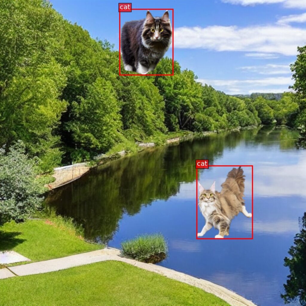
画像分類では被写体の画像とラベルさえあればいいので、背景画像からBBoxの領域を切り出して
- image
- label
を返すようなクラスにします。
また、ギリギリの範囲にならないようにbbox_marginでマージンを設定します。
import json
from pathlib import Path

import torch
from PIL import Image
from torch.utils.data import Dataset


class CocoClassificationDataset(Dataset):
    def __init__(
        self,
        image_dir,
        annotation_file,
        transform=None,
        bbox_margin=0.0,
    ):
        """
        COCO形式の物体検出データセットからBBoxで物体を切り出し、
        画像分類用データセットとして返す。

        Parameters
        ----------
        image_dir : str
            画像フォルダ
        annotation_file : str
            COCO形式のJSONファイル
        transform : callable, optional
            torchvision.transformsなど
        bbox_margin : float
            BBoxの周囲に追加する余白の割合
            例: 0.1ならBBoxサイズの10%を追加
        """

        self.image_dir = Path(image_dir)
        self.transform = transform
        self.bbox_margin = bbox_margin

        with open(annotation_file, "r", encoding="utf-8") as f:
            coco = json.load(f)

        # image_id -> 画像情報
        self.images = {
            image["id"]: image
            for image in coco["images"]
        }

        # category_id -> category名
        categories = {
            category["id"]: category["name"]
            for category in coco["categories"]
        }

        # 犬猫だけを使用
        target_categories = {
            category_id: name
            for category_id, name in categories.items()
            if name.lower() in ["dog", "cat"]
        }

        # 分類ラベルを0始まりにする
        class_names = sorted(target_categories.values())

        self.class_to_idx = {
            class_name: index
            for index, class_name in enumerate(class_names)
        }

        self.idx_to_class = {
            index: class_name
            for class_name, index in self.class_to_idx.items()
        }

        # annotation 1個 = 分類用サンプル1個
        self.samples = []

        for annotation in coco["annotations"]:
            category_id = annotation["category_id"]

            if category_id not in target_categories:
                continue

            image_id = annotation["image_id"]
            class_name = target_categories[category_id]

            self.samples.append({
                "image_id": image_id,
                "bbox": annotation["bbox"],
                "label": self.class_to_idx[class_name],
            })

    def __len__(self):
        return len(self.samples)

    def __getitem__(self, index):
        sample = self.samples[index]

        image_info = self.images[sample["image_id"]]

        image_path = self.image_dir / image_info["file_name"]

        image = Image.open(image_path).convert("RGB")

        # COCO bbox
        # [x, y, width, height]
        x, y, w, h = sample["bbox"]

        # BBox周囲の余白
        margin_x = w * self.bbox_margin
        margin_y = h * self.bbox_margin

        x1 = max(0, x - margin_x)
        y1 = max(0, y - margin_y)
        x2 = min(image.width, x + w + margin_x)
        y2 = min(image.height, y + h + margin_y)

        # PIL crop:
        # (left, upper, right, lower)
        image = image.crop((x1, y1, x2, y2))

        if self.transform is not None:
            image = self.transform(image)

        label = torch.tensor(
            sample["label"],
            dtype=torch.long,
        )

        return image, label
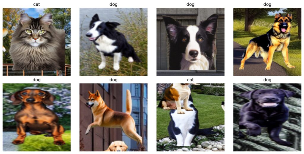
データセットクラスから画像が読み込めるか、何枚か表示して確認してみます。
import random

import matplotlib.pyplot as plt
from torch.utils.data import DataLoader
from torchvision import transforms
from dataset import CocoClassificationDataset

# ========================================
# Transform
# ========================================

transform = transforms.Compose([
    transforms.Resize((224, 224)),
    transforms.ToTensor(),
])


# ========================================
# Dataset
# ========================================

train_dataset = CocoClassificationDataset(
    image_dir="dataset/train",
    annotation_file=(
        "dataset/"
        "annotation/instances_train.json"
    ),
    transform=transform,
    bbox_margin=0.1,
)

print(f"データ数: {len(train_dataset)}")
print(f"クラス: {train_dataset.class_to_idx}")


# ========================================
# DataLoader
# ========================================

train_loader = DataLoader(
    train_dataset,
    batch_size=32,
    shuffle=True,
    num_workers=0,
)


# ========================================
# DataLoaderから1バッチ取得
# ========================================

images, labels = next(iter(train_loader))

print(f"images shape: {images.shape}")
print(f"labels shape: {labels.shape}")


# ========================================
# ランダムに画像を表示
# ========================================

num_show = 8

indices = random.sample(
    range(len(images)),
    min(num_show, len(images))
)

plt.figure(figsize=(12, 6))

for i, index in enumerate(indices):
    image = images[index]
    label = labels[index].item()

    # Tensor: [C, H, W]
    # matplotlib: [H, W, C]
    image = image.permute(1, 2, 0).numpy()

    class_name = train_dataset.idx_to_class[label]

    plt.subplot(2, 4, i + 1)
    plt.imshow(image)
    plt.title(class_name)
    plt.axis("off")

plt.tight_layout()
plt.savefig(
    "augmentation_samples.png",
    dpi=150,
    bbox_inches="tight"
)
plt.show()
実行結果はこちら。
被写体の読出しは問題なさそうですね(かぶっている部分は切り出しとは別の問題なので一旦スルーします)。
3. 前処理(Transforms)
次にtransforms、いわゆるデータ拡張処理を実装していきます。
データ拡張の種類は豊富ですが、何でもいいわけではないので、今回は代表的な
- RandomResizedCrop:拡大・縮小
- RandomHorizontalFlip:左右反転
- RandomRotation:回転
- ColorJitter:色・明るさ変更
で試していきます。
from torchvision import transforms

def get_transforms():
    transform = transforms.Compose([
        transforms.Resize((256, 256)),

        transforms.RandomResizedCrop(224, scale=(0.8, 1.0),ratio=(0.9, 1.1),),
        transforms.RandomHorizontalFlip(p=0.5),
        transforms.RandomRotation(10),
        transforms.ColorJitter(brightness=0.2, contrast=0.2, saturation=0.2, hue=0.05,),
        transforms.ToTensor(),
    ])
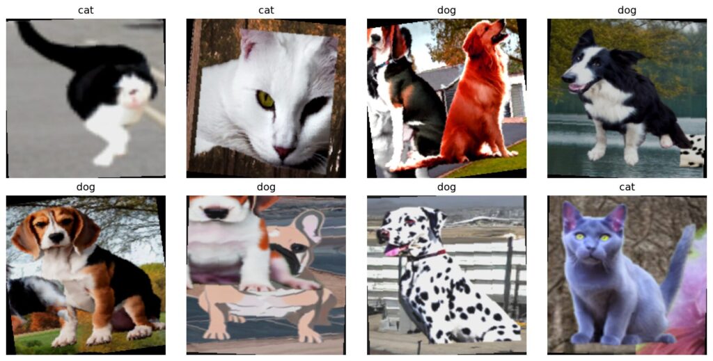
return transformデータ拡張を加えたデータセットを確認してみます。
import random

import matplotlib.pyplot as plt
from torch.utils.data import DataLoader
from torchvision import transforms
from dataset import CocoClassificationDataset
from torchvision import transforms

# ========================================
# Transform
# ========================================

transform = transforms.Compose([
    transforms.Resize((256, 256)),

    transforms.RandomResizedCrop(224, scale=(0.8, 1.0),ratio=(0.9, 1.1),),
    transforms.RandomHorizontalFlip(p=0.5),
    transforms.RandomRotation(10),
    transforms.ColorJitter(brightness=0.2, contrast=0.2, saturation=0.2, hue=0.05,),
    transforms.ToTensor(),
])

# ========================================
# Dataset
# ========================================

train_dataset = CocoClassificationDataset(
    image_dir="dataset/train",
    annotation_file=(
        "dataset/"
        "annotation/instances_train.json"
    ),
    transform=transform,
    bbox_margin=0.1,
)

print(f"データ数: {len(train_dataset)}")
print(f"クラス: {train_dataset.class_to_idx}")


# ========================================
# DataLoader
# ========================================

train_loader = DataLoader(
    train_dataset,
    batch_size=32,
    shuffle=True,
    num_workers=0,
)


# ========================================
# DataLoaderから1バッチ取得
# ========================================

images, labels = next(iter(train_loader))

print(f"images shape: {images.shape}")
print(f"labels shape: {labels.shape}")


# ========================================
# ランダムに画像を表示
# ========================================

num_show = 8

indices = random.sample(
    range(len(images)),
    min(num_show, len(images))
)

plt.figure(figsize=(12, 6))

for i, index in enumerate(indices):
    image = images[index]
    label = labels[index].item()

    # Tensor: [C, H, W]
    # matplotlib: [H, W, C]
    image = image.permute(1, 2, 0).numpy()

    class_name = train_dataset.idx_to_class[label]

    plt.subplot(2, 4, i + 1)
    plt.imshow(image)
    plt.title(class_name)
    plt.axis("off")

plt.tight_layout()

plt.savefig(
    "augmentation_transforms_samples.png",
    dpi=150,
    bbox_inches="tight"
)
plt.show()
実行結果はこちら。
他はわかりづらいですが回転しているのはわかると思います。
4. Logger
Python標準ライブラリのloggerを使えばログを保存することができます。
logフォルダを作成し、loggerの初期化を行を行うsetup_logger()を実装します。
import logging
from pathlib import Path

def setup_logger(model_name):
    log_dir = Path("logs")
    log_dir.mkdir(exist_ok=True)

    logger = logging.getLogger(model_name)
    logger.setLevel(logging.INFO)

    # 重複追加を防止
    if not logger.handlers:
        file_handler = logging.FileHandler(
            log_dir / f"{model_name}.log",
            encoding="utf-8",
        )

        console_handler = logging.StreamHandler()

        formatter = logging.Formatter(
            "%(asctime)s - %(levelname)s - %(message)s"
        )

        file_handler.setFormatter(formatter)
        console_handler.setFormatter(formatter)

        logger.addHandler(file_handler)
        logger.addHandler(console_handler)

return logger5. モデル読み込み
次にモデル読み込み用関数create_model()を実装します。
今回は4種類のモデルを試す予定なので、モデル読み込み部分を共通化し、引数でモデルを指定する形式にします。
また、今後ファインチューニングを行うことも想定し、引数にpretrainedを指定することで学習済みモデルを使用するか選択できるようにしておきます。
import torch
import torch.nn as nn

from torchvision.models import (
    vgg16,
    VGG16_Weights,
    resnet50,
    ResNet50_Weights,
    efficientnet_b0,
    EfficientNet_B0_Weights,
    convnext_tiny,
    ConvNeXt_Tiny_Weights,
)


def create_model(
    model_name,
    num_classes=2,
    pretrained=True,
):
    if model_name == "vgg16":
        weights = (
            VGG16_Weights.DEFAULT
            if pretrained else None
        )

        model = vgg16(weights=weights)

        model.classifier[6] = nn.Linear(
            model.classifier[6].in_features,
            num_classes
        )

    elif model_name == "resnet50":
        weights = (
            ResNet50_Weights.DEFAULT
            if pretrained else None
        )

        model = resnet50(weights=weights)

        model.fc = nn.Linear(
            model.fc.in_features,
            num_classes
        )

    elif model_name == "efficientnet_b0":
        weights = (
            EfficientNet_B0_Weights.DEFAULT
            if pretrained else None
        )

        model = efficientnet_b0(weights=weights)

        model.classifier[1] = nn.Linear(
            model.classifier[1].in_features,
            num_classes
        )

    elif model_name == "convnext_tiny":
        weights = (
            ConvNeXt_Tiny_Weights.DEFAULT
            if pretrained else None
        )

        model = convnext_tiny(weights=weights)

        model.classifier[2] = nn.Linear(
            model.classifier[2].in_features,
            num_classes
        )

    else:
        raise ValueError(
            f"未対応のモデルです: {model_name}"
        )

    return model
呼び出すときの処理はこちらです。
model = create_model(
    model_name=model_name,
    num_classes=num_classes,
    pretrained=pretrained,
)

model = model.to(device)6. メインの処理
ここからはメインの処理を実装していきます。
6.1. Device取得
デバイス取得です。
GPUを認識している場合は”cuda”、CPUなら”cpu”が使用されます。
device = torch.device(
    "cuda" if torch.cuda.is_available() else "cpu"
)
6.2. 損失関数
次に損失関数を実装します。
ここでは画像分類で一般的に使用されている交差エントロピーを採用します。
criterion = nn.CrossEntropyLoss()6.3. Optimizer
次にOptimizer(最適化アルゴリズム)を実装します。
今回はAdamWを採用しました。
SGDでもいいのですが、AdamWのほうがハイパーパラメータを細かく調整しなくても比較的学習が安定しやすいです。
optimizer = torch.optim.AdamW(
    model.parameters(),
    lr=learning_rate,
    weight_decay=weight_decay,
)
6.4. Scheduler
最後にスケジューラーを設定します。
今回はCosineAnnealingLRを使用します。
CosineAnnealingLRは学習率をコサイン曲線にそって徐々に小さくしていくスケジューラーです。
学習初期は大きめの学習率でパラメータを更新し、学習が進むにつれて学習率を滑らかに小さくしていきます。
StepLRのように一定間隔で学習率を下げていく方法もありますが、今回は学習率を滑らかに減少させることができるCosineAnnealingLRを採用します。
scheduler = torch.optim.lr_scheduler.CosineAnnealingLR(
    optimizer,
    T_max=num_epochs,
    eta_min=eta_min,
)7. 学習処理
次に学習処理を実装します。
ここでは
学習(train) → 検証(validation)の流れで、学習データを使ってモデルのパラメータを更新し、各epoch終了後にValidationデータで検証します。
7.1. 学習(Train)
まずは学習処理です。
def train(
    model,
    train_loader,
    criterion,
    optimizer,
    device,
):
    model.train()

    running_loss = 0.0
    correct = 0
    total = 0

    for images, labels in train_loader:
        images = images.to(device)
        labels = labels.to(device)

        # 勾配を初期化
        optimizer.zero_grad()

        # 順伝播
        outputs = model(images)

        # 損失計算
        loss = criterion(outputs, labels)

        # 逆伝播
        loss.backward()

        # パラメータ更新
        optimizer.step()

        # Loss集計
        running_loss += loss.item() * images.size(0)

        # Accuracy集計
        predicted = outputs.argmax(dim=1)

        total += labels.size(0)
        correct += (predicted == labels).sum().item()

    epoch_loss = running_loss / total
    epoch_accuracy = correct / total

    return epoch_loss, epoch_accuracy
7.2. 検証(Validation)
検証処理も同様に実装します。
こちらは順伝播とLossの計算のみです。
def validate(
    model,
    val_loader,
    criterion,
    device,
):
    model.eval()

    running_loss = 0.0
    correct = 0
    total = 0

    with torch.no_grad():
        for images, labels in val_loader:
            images = images.to(device)
            labels = labels.to(device)

            outputs = model(images)

            loss = criterion(outputs, labels)

            running_loss += loss.item() * images.size(0)

            predicted = outputs.argmax(dim=1)

            total += labels.size(0)
            correct += (predicted == labels).sum().item()

    epoch_loss = running_loss / total
    epoch_accuracy = correct / total

    return epoch_loss, epoch_accuracy
7.3. 学習用関数
学習用の関数を実装します。
def train_model(
        model,
        run_name,
        num_epochs,
        device,
        train_loader,
        val_loader,
        criterion,
        scheduler,
        optimizer,
        patience,
        logger,
):
    best_val_loss = float("inf")
    best_val_acc = 0.0
    best_epoch = 0
    early_stop_count = 0

    model_dir = Path("models")
    model_dir.mkdir(exist_ok=True)

    model_path = model_dir / f"best_{run_name}.pth"

    # ========================================
    # TensorBoard
    # ========================================

    writer = SummaryWriter(
        log_dir=f"runs/{run_name}"
    )

    logger.info("Training started")

    try:
        for epoch in range(num_epochs):

            # ========================================
            # Train
            # ========================================

            train_loss, train_acc = train(
                model=model,
                train_loader=train_loader,
                criterion=criterion,
                optimizer=optimizer,
                device=device,
            )

            # ========================================
            # Validation
            # ========================================

            val_loss, val_acc = validate(
                model=model,
                val_loader=val_loader,
                criterion=criterion,
                device=device,
            )

            # ========================================
            # TensorBoard Write
            # ========================================

            current_lr = optimizer.param_groups[0]["lr"]

            writer.add_scalar(
                "Loss/train",
                train_loss,
                epoch + 1,
            )

            writer.add_scalar(
                "Loss/val",
                val_loss,
                epoch + 1,
            )

            writer.add_scalar(
                "Accuracy/train",
                train_acc,
                epoch + 1,
            )

            writer.add_scalar(
                "Accuracy/val",
                val_acc,
                epoch + 1,
            )

            writer.add_scalar(
                "LearningRate",
                current_lr,
                epoch + 1,
            )

            # ========================================
            # Scheduler
            # ========================================

            scheduler.step()

            # ========================================
            # 結果表示
            # ========================================

            logger.info(
                f"Epoch [{epoch + 1:03d}/{num_epochs}] "
                f"Train Loss: {train_loss:.4f} "
                f"Train Acc: {train_acc:.4f} | "
                f"Val Loss: {val_loss:.4f} "
                f"Val Acc: {val_acc:.4f} | "
                f"LR: {current_lr:.8f}"
            )

            # ========================================
            # Best Model Save
            # ========================================

            if val_loss < best_val_loss:
                best_val_loss = val_loss
                best_val_acc = val_acc
                best_epoch = epoch + 1
                early_stop_count = 0

                torch.save(
                    model.state_dict(),
                    model_path,
                )

                logger.info(
                    f"Best Epoch: {best_epoch} | "
                    f"Val Loss: {best_val_loss:.4f} | "
                    f"Val Acc: {best_val_acc:.4f}"
                )

            else:
                early_stop_count += 1

                logger.info(
                    f"EarlyStopping: "
                    f"{early_stop_count}/{patience}"
                )

            # ========================================
            # Early Stopping
            # ========================================

            if early_stop_count >= patience:
                logger.info(
                    f"Early stopping at epoch {epoch + 1}"
                )
                break
    finally:
        writer.close()

    logger.info("Training finished")
    logger.info(
        f"Best Result | "
        f"Epoch: {best_epoch} | "
        f"Val Loss: {best_val_loss:.4f} | "
        f"Val Acc: {best_val_acc:.4f}"
    )
7.3.1. TensorBoard
ここでSummaryWriterを定義し、TensorBoardで学習状況を可視化できるようにしておきます。
writer = SummaryWriter(
    log_dir=f"runs/{run_name}"
)
TensorBoardはこちらのコマンドでインストールできます。
pip install tensorboard以下の処理で、trainとvalidationのLossとAccuracy、学習率を記録します。
current_lr = optimizer.param_groups[0]["lr"]

writer.add_scalar(
    "Loss/train",
    train_loss,
    epoch + 1,
)

writer.add_scalar(
    "Loss/val",
    val_loss,
    epoch + 1,
)

writer.add_scalar(
    "Accuracy/train",
    train_acc,
    epoch + 1,
)

writer.add_scalar(
    "Accuracy/val",
    val_acc,
    epoch + 1,
)

writer.add_scalar(
    "LearningRate",
    current_lr,
    epoch + 1,
)
7.3.2. Best Modelの保存
学習途中のBest Model(ValidationのLossが最小になったモデル)を保存しておき、学習終了時点で最後に保存されていたモデルを学習結果として出力します。
if val_loss < best_val_loss:
            best_val_loss = val_loss
            best_val_acc = val_acc
            best_epoch = epoch + 1
            early_stop_count = 0

            torch.save(
                model.state_dict(),
                model_path,
)7.3.3. Early Stopping
Validation Lossが一定epoch改善しなくなった場合、それ以上学習を続けてもValidation性能の改善が期待しにくいと判断し、早期終了(Early Stopping)を入れて学習を終了するように設定しておきます。
例えばpatience=10に設定されていれば、Validation Lossの最小値が10回連続で更新されなかったらその時点で学習を終了します。
if early_stop_count >= patience:
            logger.info(
                f"Early stopping at epoch {epoch + 1}"
            )
break8. ベストモデル検証
最後に学習終了時点のBest Modelで検証データのLossとAccuracyを計算し、モデルの精度を確認します。
import torch
from pathlib import Path
from train import validate

def evaluate_best_model(
    model,
    run_name,
    val_loader,
    criterion,
    device,
    logger,
):
    # ========================================
    # Bestモデル読み込み
    # ========================================

    model_path = (
        Path("models")
        / f"best_{run_name}.pth"
    )

    model.load_state_dict(
        torch.load(
            model_path,
            map_location=device,
            weights_only=True,
        )
    )

    model = model.to(device)

    # ========================================
    # Validation
    # ========================================

    val_loss, val_acc = validate(
        model=model,
        val_loader=val_loader,
        criterion=criterion,
        device=device,
    )

    logger.info("\n===== Best Model Result =====")
    logger.info(f"Model:    {run_name}")
    logger.info(f"Val Loss: {val_loss:.4f}")
    logger.info(f"Val Acc:  {val_acc:.4f}")

return val_loss, val_acc9. 実際に学習させてみる
ここからは実際に学習させてみます。
今回は犬・猫それぞれ100匹ずつ、背景1000枚生成し、train80%、val20%の割合でデータセットを作成しました。
また今回指定したパラメータはこちら
| 項目 | パラメータ | 備考 |
|---|---|---|
| Model | ResNet50 | |
| Batch size | 32 | |
| Epoch | 100 | |
| Patience | 10 | |
| Learning rate | 0.001 | AdamWデフォルト |
| Weight decay | 0.01 | AdamWデフォルト |
| Eta min | 1e-06 | デフォルト値は0。 学習終盤でも小さなパラメータ更新を継続するため最小学習率を設定 |
| Device | CUDA |
2026-08-16 13:34:49,307 - INFO - Run: resnet50_20260816_133449
2026-08-16 13:34:49,324 - INFO - ===== Training Configuration =====
2026-08-16 13:34:49,324 - INFO - Model: resnet50
2026-08-16 13:34:49,324 - INFO - Pretrained: False
2026-08-16 13:34:49,325 - INFO - Batch size: 32
2026-08-16 13:34:49,325 - INFO - Epochs: 100
2026-08-16 13:34:49,325 - INFO - Patience: 10
2026-08-16 13:34:49,325 - INFO - Learning rate: 0.001
2026-08-16 13:34:49,325 - INFO - Weight decay: 0.01
2026-08-16 13:34:49,325 - INFO - Eta min: 1e-06
2026-08-16 13:34:49,325 - INFO - Device: cuda
2026-08-16 13:34:49,449 - INFO - train data: 2332
2026-08-16 13:34:49,449 - INFO - val data:   591
2026-08-16 13:34:49,449 - INFO - class:      {'cat': 0, 'dog': 1}
2026-08-16 13:34:49,682 - INFO - model: resnet50
2026-08-16 13:34:49,682 - INFO - pretrained: False
2026-08-16 13:34:49,683 - INFO - optimizer: AdamW
2026-08-16 13:34:49,683 - INFO - scheduler: CosineAnnealingLR
2026-08-16 13:34:49,684 - INFO - Training started
2026-08-16 13:35:16,428 - INFO - Epoch [001/100] Train Loss: 0.7688 Train Acc: 0.6231 | Val Loss: 0.5826 Val Acc: 0.6819 | LR: 0.00100000
2026-08-16 13:35:16,504 - INFO - Best Epoch: 1 | Val Loss: 0.5826 | Val Acc: 0.6819
2026-08-16 13:35:42,911 - INFO - Epoch [002/100] Train Loss: 0.5662 Train Acc: 0.7204 | Val Loss: 1.5519 Val Acc: 0.7174 | LR: 0.00099975
2026-08-16 13:35:42,911 - INFO - EarlyStopping: 1/10
2026-08-16 13:36:09,075 - INFO - Epoch [003/100] Train Loss: 0.4975 Train Acc: 0.7719 | Val Loss: 0.6639 Val Acc: 0.7022 | LR: 0.00099901
2026-08-16 13:36:09,075 - INFO - EarlyStopping: 2/10
2026-08-16 13:36:35,219 - INFO - Epoch [004/100] Train Loss: 0.4698 Train Acc: 0.7864 | Val Loss: 0.4201 Val Acc: 0.8342 | LR: 0.00099778
2026-08-16 13:36:35,300 - INFO - Best Epoch: 4 | Val Loss: 0.4201 | Val Acc: 0.8342
2026-08-16 13:37:01,666 - INFO - Epoch [005/100] Train Loss: 0.3918 Train Acc: 0.8268 | Val Loss: 0.3108 Val Acc: 0.8731 | LR: 0.00099606
2026-08-16 13:37:01,822 - INFO - Best Epoch: 5 | Val Loss: 0.3108 | Val Acc: 0.8731
学習は順調に進んでいるように見えるかもしれませんが、1エポックが妙に遅いです。
ログを見てみると、1エポック約26秒ほどかかっています。
今回の検証PCは5070tiを積んでいるのでこの程度ならもっと早いイメージです。
もしやと思いタスクマネージャーを見てみたら
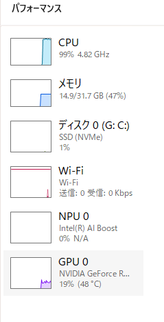

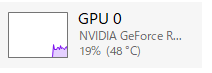
CPUの使用率が極限に達していてGPUが20%しか使われていませんでした。
おそらく学習の前段階でCPU処理がボトルネックになっているのでしょう。
この状態でも時間をかければ学習は完了するかもしれませんが、効率が悪いのでいったん学習を中断しました。
10. まとめ
今回、AI画像で作成したデータセットで画像分類を試してみるために学習プログラムを実装し、学習を実行してみました。
しかしCPU処理がボトルネックになっていることが判明し、GPUがほとんど使われず学習に時間がかかりそうだったのでいったん中断しました。
次回はCPU処理の速度を改善し、GPUをフルで使用できるようにして改めて検証していきたいと思います。

11. 参考サイト
Datasets & DataLoaders
https://docs.pytorch.org/tutorials/beginner/basics/data_tutorial.html
CrossEntropyLoss
https://docs.pytorch.org/docs/2.13/generated/torch.nn.CrossEntropyLoss.html
AdamW
https://docs.pytorch.org/docs/2.13/generated/torch.optim.AdamW.html
CosineAnnealingLR
https://docs.pytorch.org/docs/2.13/generated/torch.optim.lr_scheduler.CosineAnnealingLR.html
Saving and Loading Models
https://docs.pytorch.org/tutorials/beginner/saving_loading_models.html
torch.utils.tensorboard
https://docs.pytorch.org/docs/2.13/tensorboard.html
12. 関連書籍
PyTorchを基礎から学ぶならこちらの書籍がおすすめです。

コメント